Suppose that our control system is made up of two subsystems. Let A be the number of critical faults in the first subsystem and let B be the number of critical faults in the second subsystem. Suppose that
A = {a1,a2,a3} where a1=0, a2=1, a3=”>1″
B = {b1,b2,b3} where b1=0, b2=1, b3=”>1″
If we are interested in the overall number of critical faults in the system, then we speak about the joint event A and B. We write the probability of this event as P(A,B).
P(A,B) is called the joint probability distribution of A and B. Specifically, P(A,B) is the set of probabilities:
{P(a1, b1), P(a1, b2), P(a1, b3), P(a2, b1), P(a2, b2), P(a2, b3), P(a3, b1), P(a3, b2), P(a3, b3)}
If we know the joint probability distribution P(A,B) then we can calculate P(A) by a formula (called marginalisation) which comes straight from the third axiom, namely:
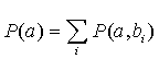
This is because the events (a,b1), (a,b2), …, (a,bm) are mutually exclusive. When we calculate P(A) in this way from the joint probability distribution we say that the variable B is marginalised out of P(A,B). It is a very useful technique because in many situations it may be easier to calculate P(A) from P(A,B).